7.4 Adjustable Plots
Adjustable plots make use of variable definitions that have been added to the plotter. When the elaboration is changed, the expression bound to the definition changes as well.
A real variable definition is displayed as a one-dimensional plot: a point on the X-axis. The value of the elaboration is indicated by a magnitude indicator. Changing the indicator by sliding it changes the elaboration.
A point variable definition is displayed as a point indicator in two-dimensional space. Changing the point indicator by dragging it in any direction changes the elaboration of the variable definition.
When variables referenced by a plottable expression are displayed in the
plotter, changes to magnitude and point indicators cause
the function to be re-evaluated.
Variables with indicators are called
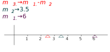
7.4.1 Adjusting magnitude
Figure 7.2 shows three magnitude adjusters, one of which is associated
with a real definition 
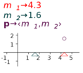
7.4.2 Adjusting a position vector
Figure 7.3 shows two magnitude adjusters and a position vector dependent on them. As the indicators are moved, the end point of the vector is changed.

7.4.3 Adjusting a point
Figure 7.4 shows a point indicator associated with a vector definition that is dependent on two real definitions, each in turn associated with magnitude indicators. Moving either of the magnitude indicators changes the position of the point indicator. Moving the point indicator itself changes the associated vector definition, losing its dependence on the real definitions.
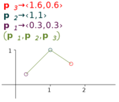
7.4.4 Adjusting line segments
Figure 7.5 shows a tuple dependent on three point indicators. Moving any of the point indicators adjusts the position of the line segments.
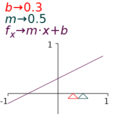
7.4.5 Adjusting a straight line
The function for a straight line is given by 


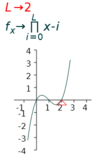
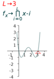
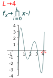
7.4.6 Adjusting the number of roots
The expression


|
|
|
| (a) 3 roots | (b) 4 roots | (b) 5 roots |
7.4.7 Adjusting a tangent
To plot a function and its tangent under the control of an adjuster,
- Add the function in the form y(x)→… to the display, say

y(x)→x^3-x . - Add the equation
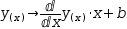
y(x)→ⅆy(x)ⅆx⋅x+b , isolate b, substitute both occurrences of y(x), take the derivative and simplify the equation. - Add an equation of the form
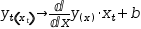
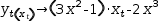
y_t(x_t)→ⅆy(x)ⅆx⋅x_t+b ; substitute y(x) and b, take the derivative and simplify. - Add a definition of the form

x→1 to the display - Select all and apply Plot. Refer to Figure 7.8.
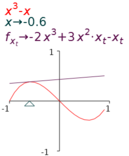 |
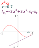 |
| (a) Tangent at x=-0.6 | (b) Tangent at x=0.7 |
Try this for (1) 
There are some issues of scope and binding that require explanation in
order to fully understand what is happening. The x in (1) is bound to
the parameter in


Try to plot the function and its tangent for
